Owning the Inference Path: 2.5× on Z-Image in Seven Triton Kernels

Context

Narcis is a project that uses diffusion models and face conditioning to produce portraits that preserve facial features. In an earlier article I explained how the first version was built, using a two-stage process: a base generation and a face-area differential diffusion.

It was built on SDXL, a well-established open-weights model that pioneered the field. Its community converged on a rich set of methods — LoRAs, ControlNets, schedulers, prompt engineering — but none of them touched the inference compute itself. For a reason: SDXL’s UNet is too irregular for systematic fusion, and its conditioning is so weak that seeds, the random noise initiating the latent at the start of the process, carry more weight on the output than most tokens in the prompt.

No surprise either: the two CLIP text encoders are architecturally outdated, providing the model with a narrow, imprecise view of what it was trained on. Optimization effort went into working around the model, not into the model’s computation. Flux, built by the former makers of SDXL, embodied the shift away from these old encoders and from the UNet architecture. Their results are far more precise, far more driven by text conditioning. The catch: the weights aren’t open. Or not fully: they eventually released a smaller version, while the interesting capacity remained API-gated.

Then came Z-Image. Released by Alibaba’s Tongyi-MAI lab, it implements this same DiT architecture while leveraging already-proven assets: the Qwen text encoder (from another team inside Alibaba) and the Flux latent decoder. A 6.15 billion parameter single-stream transformer, fully open weights, with conditioning that actually works.

This was the architecture and the open-source commitment I was waiting for.

Outline

Libraries are general tooling, and the price for that generality is at every call site. When you have fixed hardware, a single model, and the willingness to go deeper, you can skip every layer that was written for someone else’s problem.

This article is about doing exactly that. I run a 6.15B-parameter diffusion transformer on NVIDIA L4 GPUs, a chip with native fp8 tensor cores that the standard diffusion tooling leaves unused. The model runs in production on AWS g6 instances. Compute is scarce, and every millisecond of inference is money.

I cut the per-step inference time from 1.75 seconds to 0.687 seconds, 2.5x, without changing the model. No new architecture, no distillation, no quantization-aware training. The method was:

1. Profile the model on the actual production hardware. Discover that the bottleneck is not where you expect.
2. Strip the inference path to its essential operations. Remove every library that exists to handle cases you don’t have.
3. Use torch.compile as a teacher, not as a solution. Read the code Inductor generates. Understand what it fuses and what it leaves on the table.
4. Write owned Triton kernels that fuse everything between the GEMMs and the attention, fp8 end-to-end, targeting the L4’s sm89 instruction set.
5. Verify every kernel numerically against an oracle, at production dimensions, with three quantitative gates.
6. Iterate until the entire inference loop runs on owned code, and the compiler itself becomes unnecessary.

The result: seven custom kernels that absorbed what PyTorch’s compiler contributed, then exceeded it. torch.compile, post-collapse, actually regresses performance: 0.701 seconds versus 0.687 seconds eager. The handwritten kernels beat the compiler.

But speed was only half the point. Owning the inference path means owning the surface. LoRA hot-swap without PEFT. Training backward passes on the same fp8 arithmetic. Production features implemented at the kernel level, not shimmed on top of a library that wasn’t designed for them. The assertion of ownership is as important as the acceleration: inference is one direction, and the others are already in progress.

The model

To understand why this optimization was possible, and why it wouldn’t have been on SDXL, you need to see the difference between a UNet and a DiT.

SDXL’s UNet is a tree. It has downsampling stages, upsampling stages, skip connections between them, and cross-attention layers where text conditioning is injected. Each stage operates at a different spatial resolution. The result is an irregular computation graph: no two layers do the same thing in the same shape. Writing a kernel that fuses operations across this structure means writing a different kernel for every stage. The effort doesn’t compound.

Z-Image’s transformer is a stack. Thirty identical blocks, one after another, bracketed by two pairs of small refiner blocks (context and noise) with the same shape and a slightly different transition structure. Each block takes the same input shape (a sequence of 3840-dimensional tokens) and produces the same output shape. Text and image tokens are concatenated into a single sequence and processed together through self-attention, with no cross-attention pathway. Conditioning enters through a lightweight adaLN mechanism: a small embedding modulates the normalization scales and gates at each block.

This regularity is the precondition for everything that follows. One kernel that fuses the operations inside a block covers all thirty blocks. The effort compounds.

A few architectural details that matter for optimization:

The text encoder is Qwen3-4B, a 4-billion parameter causal language model producing 2560-dimensional features over up to 512 tokens. Compare this to SDXL’s CLIP encoders, which cap at 77 tokens and whose representation capacity was already stale when SDXL shipped. The Qwen encoder is why Z-Image actually follows its prompts.

The VAE is borrowed from Flux: 16-channel latents at a scale factor of 8. SDXL uses 4 channels. More latent channels means a richer compressed representation of the image, which translates directly into finer detail in the decoded output.

The prediction method is flow matching with velocity prediction. Where SDXL learns to predict noise (epsilon prediction) and requires 20 to 50 denoising steps with a beta schedule, Z-Image learns to predict the velocity along a straight trajectory from noise to data. The noising formula is x_t = (1 - sigma) * x0 + sigma * noise, and the model predicts v = x0 - noise. Straight trajectories mean fewer steps: 9 in production, with no classifier-free guidance (the model is CFG-distilled). This alone makes Z-Image 3 to 5 times cheaper per image than SDXL at equivalent resolution.

The block structure, unrolled, is a sequence of well-defined operations between six GEMMs and one attention call:

RMSNorm → adaLN modulate → FP8 quant → Q/K/V projections (3 GEMMs) → QK-RMSNorm + 3-axis RoPE
  → Scaled Dot-Product Attention → permute + FP8 quant → output projection (GEMM) → residual
  → RMSNorm → adaLN modulate → FP8 quant → w1/w3 projections (2 GEMMs) → SiLU gate → FP8 quant
  → w2 projection (GEMM) → gate + residual → next block

The GEMMs and the attention are already hardware-optimal: CUTLASS sm89 kernels for fp8 matrix multiplies, fmha_cutlassF for attention. These are what NVIDIA spent years optimizing. You don’t rewrite them.

Everything between them was not optimal. Every RMSNorm decomposed into pow, mean, rsqrt as three separate CUDA launches. Every dtype conversion materialized an intermediate tensor to global memory. Every modulation a separate elementwise pass. These operations, collectively, consumed 35% of GPU time. That 35% was the target.

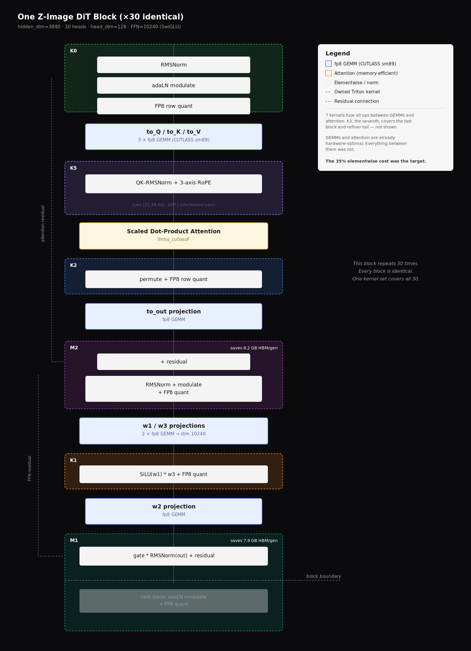One Z-Image DiT block, repeated thirty times. The blue GEMMs and the attention are already hardware-optimal; the shaded regions (K0, K5, K2, M2, K1, M1) are the owned kernels that fuse everything between them. The seventh, K3, covers the last block and refiner tail. This regularity is what makes one kernel set cover all thirty blocks.

The hardware

The model runs on NVIDIA L4 GPUs, deployed on AWS g6.xlarge instances. The L4 is an Ada Lovelace chip (sm89, compute capability 8.9): 24 GB GDDR6, 300 GB/s memory bandwidth, 72 watts. It is a cost-efficient inference GPU, not a training GPU. It is also, for this work, the right one.

The reason is fp8. Ada Lovelace introduced native fp8 tensor cores: 242 dense TFLOPS in float8_e4m3fn, twice the dense throughput of bf16 on the same silicon (242 versus 121 TFLOPS). Most inference workloads on L4 run in bf16 or int8.

The diffusion ecosystem in particular has no built-in fp8 path: the diffusers library runs DiTs in bf16 by default. And fp8 on sm89 is not something to take on faith: torch._scaled_mm accepting fp8 inputs does not prove the GEMM ran at fp8 speed. The profiler had to confirm the dispatch — CUTLASS sm89 kernel names in the trace, not a quiet fallback.

I went fp8 end-to-end: both weights and activations quantized to float8_e4m3fn (max representable value: 448.0). The seven block-linear projections (to_q, to_k, to_v, to_out, w1, w2, w3) are quantized at load time. Activations are quantized dynamically at each kernel boundary, with per-token row scaling. Embedders, adaLN parameters, and the final output layer remain in bf16 as they are small and precision-sensitive.

The quantization scheme is rowwise: one scale per output channel for weights, one scale per token for activations. The alternative, tensorwise, uses a single scale per entire tensor and is about 8% faster on this hardware (cuBLASLt versus CUTLASS sm89). But rowwise is not a performance choice: it is a compatibility constraint. The owned kernels fuse quantization into the producing operation, computing each row’s scale locally as the data is generated. Tensorwise requires a global scale over the entire tensor, which cannot be computed inside a fused kernel without a separate reduction pass, defeating the fusion. torch._scaled_mm with rowwise scales dispatches to CUTLASS sm89; tensorwise dispatches to cuBLASLt. The owned kernels only compose with the rowwise path.

The memory arithmetic matters. The Z-Image transformer in bf16 weighs approximately 12.3 GB (6.15B parameters x 2 bytes). In fp8, the seven quantized linear projections shrink to roughly 6.2 GB, with the remaining bf16 parameters (embedders, norms, adaLN) adding about 0.5 GB. Total model footprint under fp8: approximately 6.7 GB. Production VRAM at inference, including activations, the Qwen encoder, and the VAE: 17.47 GB out of 24 GB available. In bf16, this model does not fit on an L4 with room for activations. In fp8, it fits comfortably.

But the memory saving is only half the story. Going fp8 end-to-end also changes the compute graph’s texture. When weights and activations are both fp8, the GEMM inputs are already in the right dtype for the tensor core. There is no bf16-to-fp8 cast before the multiply, and no fp8-to-bf16 cast after. The tensor core consumes fp8 and returns bf16, which the next owned kernel immediately re-quantizes to fp8 for the next GEMM. The dtype conversion overhead that consumed part of that 35% elementwise cost disappears: it is absorbed into the kernel that produces the activation, not executed as a standalone CUDA launch.

This is the hardware thesis of the entire optimization: one chip, one instruction set, one memory budget. Every kernel targets sm89 CUTLASS rowwise _scaled_mm. Every fusion decision is made with 24 GB of GDDR6 as the ceiling. Every intermediate tensor that can stay in L2 or registers instead of round-tripping to global memory is a win, because at 300 GB/s, memory bandwidth is the wall that all the 242 TFLOPS of fp8 compute are pressing against.

This code is not portable. It is written for this chip, and it ships on this chip.

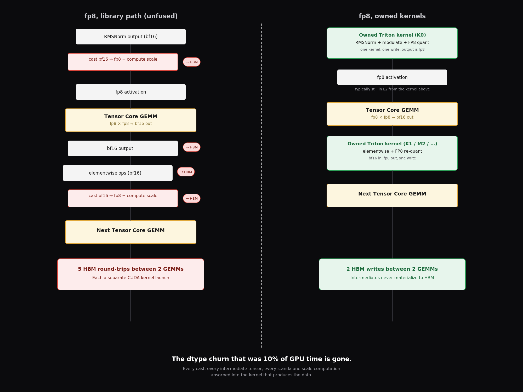The fp8 data path. Left: the library path round-trips through HBM five times between two GEMMs, each a separate CUDA launch. Right: the owned kernels write twice — intermediates never materialize to HBM. The dtype churn that was ~10% of GPU time disappears.

The method

To me, this is the most important part of the work. I went into this knowing I was past the edge of what I understood, learning as I went. That meant I needed a disciplined framework: how to analyze, assess, quantify, and validate at each step. There were many places where a wrong turn could send me into a depth of problems I would not have been able to surface from. Structured thinking from the first step gave me clarity for every decision that followed.

This section is how the work was done.

Profiling

The first step was to measure. I instrumented a production inference pass: 9 steps at 832x1216 resolution, clocks locked at 1830 MHz, on the target L4. The torch profiler traced 15,952 GPU events across 4 active steps, covering 7,298 ms of GPU time with 100% attribution (0.04 ms unattributed).

The results contradicted the obvious hypothesis.

The nf4 quantization tax, the thing I expected to dominate, was 3.1%. The dequantization kernel (kDequantizeBlockwise) and its 4-bit gemv were a rounding error, not a bottleneck. GPU idle time inside the traced window was 0.5%, meaning CUDA graph capture, the standard remedy for launch overhead, would save almost nothing.

The actual breakdown:

• GEMM: 41.2%. Matrix multiplications, already dispatched to tensor cores. Not the target.
• Attention: 20.3%. fmha_cutlassF, memory-efficient backend. Also not the target.
• Elementwise and normalization: 35.3%. This was the start of the thread to unravel.

Inside that 35%, the anatomy was revealing. RMSNorm was never fused: pow, mean, rsqrt each launched as separate CUDA kernels, 820 calls each across the trace (roughly 205 per step, once per block per operation). The mul kernel fired 2,580 times for 844 ms. The copy_ kernel, which is pure dtype conversion overhead, fired 2,264 times for 739 ms, consuming roughly 10% of total GPU time by itself. The single most expensive non-GEMM kernel was pow_tensor_scalar at 442 ms (6% of GPU time), a component of RMSNorm that exists only because PyTorch decomposes x * rsqrt(mean(x^2) + eps) into four separate operations.

Step time was flat across all 9 steps (min 1.681s, max 1.796s), confirming that no step has special structure worth exploiting. The inference loop is uniform. The optimization is uniform.

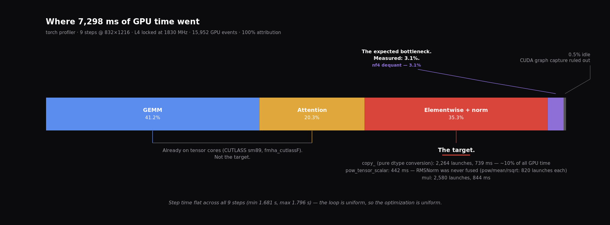Where 7,298 ms of GPU time went. GEMM and attention are already on tensor cores — not the target. The nf4 dequant tax I expected to dominate measured 3.1%, and idle time was 0.5%, ruling out CUDA graphs. The 35.3% elementwise and norm band — copy_, pow, mul — was the target.

Trimming

Before writing any kernel, I stripped the inference path. The goal was to reduce the graph to its essential operations, removing every library layer that existed to handle hardware or configurations I don’t have.

The vendored transformer was the largest single change: I forked the diffusers implementation of the Z-Image S3-DiT into our own codebase. This eliminated 74 graph breaks that torch.compile could not trace through, caused by dynamic dispatch, logging, and compatibility code inside diffusers. With the vendored transformer, the entire forward pass is a single traceable graph.

The nf4 quantization path (bitsandbytes) was removed entirely. It had served its purpose as the initial deployment strategy, but fp8 made it obsolete. With it went the dequantization kernels, the 4-bit gemv fallback, and the associated memory choreography.

PEFT, the library for LoRA weight management, was next. Its abstraction layer intercepts every linear forward call to check for active adapters, compute the low-rank delta, and merge it into the output. This interception happens at every call, whether or not the adapter has changed. I replaced it with an owned LoRA module that preserves runtime hot-swap but eliminates the per-forward overhead. The mechanism uses preallocated buffers and copy_ operations: swapping a LoRA for a different subject is a buffer copy into fixed-shape tensors, not a re-trace of the graph. The forward path sees only the base fp8 GEMM plus a static low-rank side-branch. No adapter registry, no per-call dispatch, no Python branches on tensor values.

Each removal simplified the graph, made the remaining operations more visible, and brought the code closer to a straight sequence of operations between GEMMs.

Compile as teacher

With a clean, traceable graph, I ran torch.compile in mode=default with Inductor as the backend. The purpose was not to ship the compiled code. It was to read what Inductor did.

Inductor is PyTorch’s graph compiler. When it works, it lowers the computation graph into fused Triton kernels, merging operations that PyTorch’s eager mode executes as separate CUDA launches. It handles operator fusion, memory planning, and code generation. The output is a directory of generated Triton source files, readable if you know what to look for.

This is worth pausing on. Inductor’s backend for CUDA does not generate C++ or PTX. It generates Python functions decorated with @triton.jit. The same language, the same framework I would later write my own kernels in. I was reading Triton from the beginning, before I knew I would be writing it.

I read every generated kernel: which operations it fused, which it left as separate launches, what dtype conversions it inserted, what memory access patterns it chose. Inductor’s fusions were the starting point. It showed me what was fusible in principle, and where its heuristics stopped short.

The constraints of using torch.compile as a production path were also instructive. The model accepts variable-length prompt sequences (the Qwen encoder tokenizes to different lengths per prompt), and Inductor traces a separate specialized graph for each unique tensor shape. In production, this means either padding all prompts to the maximum length (wasting compute) or pre-compiling at container start for a discrete set of sequence lengths. I bucketed prompt lengths into a small set of padded slots (64, 128, 192 tokens), each slot requiring its own compile pass at cold start. With Inductor’s warmup costing on the order of 100 seconds per shape on the L4, container start time became a deployment constraint.

This was one of the reasons the compiled path was ultimately replaced. But the code it generated remained the teacher.

Fusion design

Armed with the profiling data and the compiler’s output, I identified the fusion targets. The principle was simple: every operation between two GEMMs (or between a GEMM and the attention) that can be computed in a single pass over the data should be computed in a single pass.

A fused kernel reads its input from global memory once, performs all the intermediate operations in registers or shared memory, and writes the final result back once. The unfused version reads and writes for every operation in the chain. On a chip where memory bandwidth (300 GB/s) is the binding constraint against the compute throughput (242 TFLOPS), eliminating memory round-trips is where the time is.

The fusion targets mapped directly onto the block diagram from The model, each region shaded onto the operations it absorbs:

• K0 (rmsnorm_modulate_fp8_quant): fuses the pre-attention RMSNorm, the adaLN scale/shift modulation, and the fp8 row quantization for the Q/K/V projections. What was three CUDA launches plus a dtype cast becomes one kernel. It de-triplicates the activation quantization: the same normalized-and-modulated tensor is quantized once and fed to all three QKV GEMMs.
• K5 (fused_qknorm_rope): fuses the post-projection QK normalization (two separate RMSNorms) with the 3-axis rotary position embedding. The RoPE implementation uses the GPT-J interleaved-pairs convention with axes_dims [32, 48, 48] on head_dim 128. What was 6 to 8 intermediate tensors (norm, scale, rotate-even, rotate-odd, interleave, per axis) becomes one kernel that reads Q and K and writes the rotated, normalized versions directly.
• K2 (attn_output_fp8_quant): fuses the attention output permute with the fp8 row quantization for the output projection GEMM.
• M2 (ffn_prologue_mega): the largest fusion. It takes the attention output, adds the residual, applies the FFN input RMSNorm, modulates via adaLN, and quantizes to fp8 for the w1/w3 GEMMs. This saves 30.4 MB per block per step from never materializing the intermediate normalized tensor at dimension 3840. Across 30 blocks and 9 steps: 8.2 GB of HBM writes that never happen.
• K1 (silu_gate_fp8_quant): fuses the SiLU activation on w1’s output, the element-wise multiply with w3’s output, and the fp8 quantization for the w2 GEMM. This eliminates a 10240-wide bf16 intermediate, the FFN hidden dimension, which in the unfused path would round-trip through global memory.
• M1 (block_transition_mega): fuses the FFN residual connection, the output gate multiplication, the RMSNorm, and the transition to the next block’s adaLN fold.
• K3 (rmsnorm_gate_residual): handles the last block and noise refiner path, where the block transition structure differs slightly from the main stack.

Oracle testing

Every kernel was verified numerically before it replaced the eager path.

The oracle methodology works as follows. Synthetic tensors are generated at production dimensions (N=3952 tokens for an 832x1216 image, D=3840 hidden dimension, head_dim=128 for the QK kernels). The kernel under test is run on these inputs. Its output is compared against the eager fp32 composition: the mathematically ideal result, computed in full precision, not the production dtype flow.

Three gates must pass:

• Gate 1 — scale accuracy. The per-row fp8 scales computed by the kernel must match the reference scales within a relative tolerance of 1e-3. This verifies that the amax computation (the row-wise maximum absolute value used to set the fp8 scale) is numerically correct.
• Gate 2 — bit-match fraction. The quantized fp8 output must exactly match the reference fp8 quantization on at least 99% of all values. For K0 on production dimensions, this means 99.59% exact bit-match across roughly 15 million fp8 values. The remaining 0.41% differ by exactly one fp8 ULP, caused by rounding-mode differences in the fused computation path.
• Gate 3 — dequantized error. The maximum absolute difference when both outputs are dequantized back to bf16 must be within one fp8 step at the top of the represented range. For K0, this was 0.958, which is one ULP at the scale of the largest values.

The oracle tests run on GPU, at production dimensions, with production dtypes. They are not unit tests against toy inputs. They verify the kernel at the exact operating point where it will run in production.

Full-generation validation, once the kernels pass their oracles, is done by quality gallery: visual output reviewed across varied prompts and subjects. Pixel-level parity is not the gate for the integrated system; numerical parity is the gate for individual kernels. Some kernel substitutions did change the output on reference seeds without any quality degradation, confirming that the oracle’s tolerance is correctly calibrated: tight enough to catch errors, loose enough to permit legitimate rounding differences.

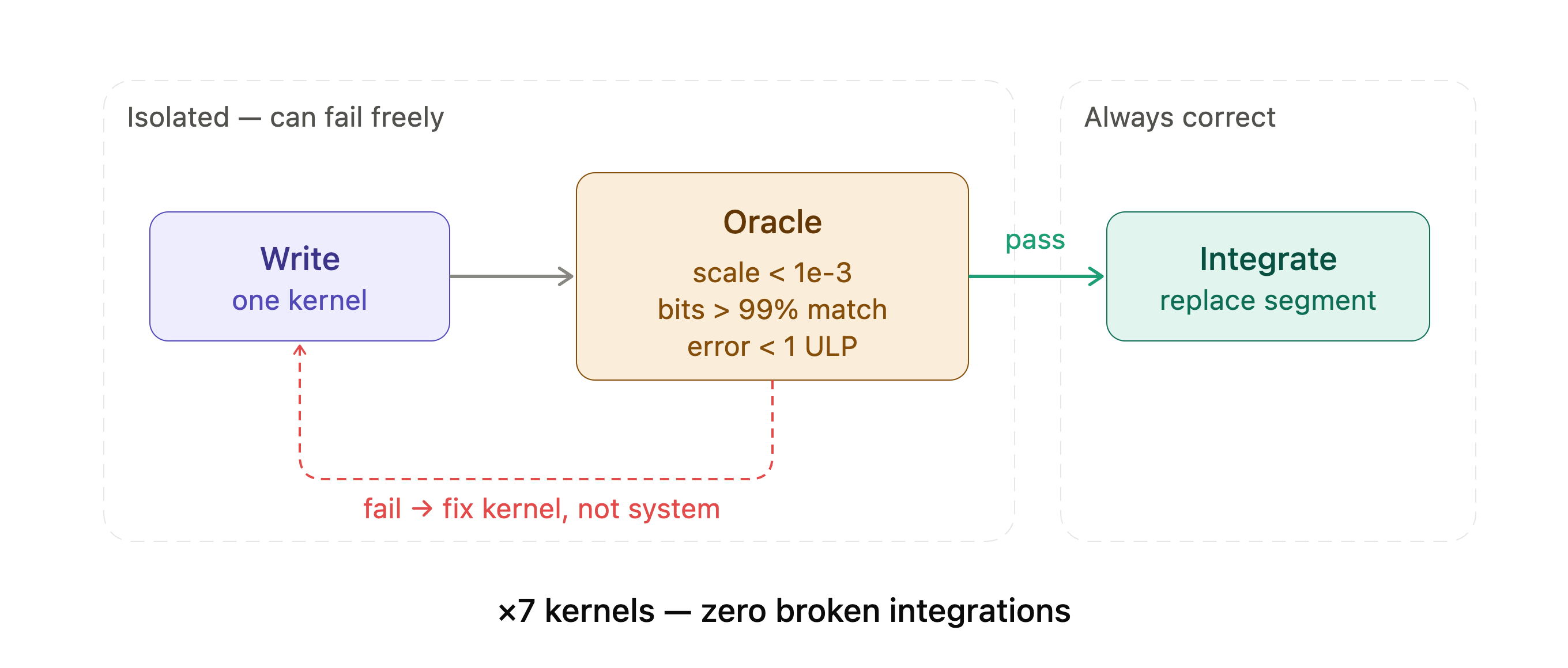The oracle as a firewall. Each kernel is developed in isolation where it can fail freely, and must clear three numerical gates before it is allowed to replace a segment of the production path. A failure loops back to fixing the kernel, never the system — across all seven kernels, zero broken integrations.

Iteration

The kernels were not written all at once. They were built one at a time, verified by the oracle, and integrated into the inference loop incrementally. Each kernel replaced one segment of the eager path while the rest continued to run through PyTorch or through the compiler.

The final step was flag collapse: removing the conditional gates that allowed falling back to the unfused path. Once all seven kernels had passed every oracle gate and the quality gallery was approved, every kernel became unconditional. The inference loop no longer had a fallback path. The flags were deleted, not turned off.

At that point, torch.compile was re-benchmarked. With all seven owned kernels unconditional, Inductor had nothing left to contribute: the operations it had been fusing were already fused by hand. The compiled path now added only Inductor’s overhead (graph capture, code generation, cache management) with no fusion benefit. The result: 0.701 seconds per step compiled versus 0.687 seconds eager. A regression. torch.compile was removed from the production path.

The kernels

A common misconception: writing GPU kernels means writing CUDA C++, compiling against the toolkit, debugging with cuda-gdb. That is the CUDA experience. It is not what happened here.

The seven kernels are Python files. Each is a function decorated with @triton.jit. Triton is OpenAI’s compiler framework for GPU programming: you write in a Python dialect that operates on blocks of data, and the compiler handles the mapping to hardware. The programmer thinks in tiles and reductions, not in warps and lanes. The kernels ship as .py files in the application repository, compiled at first call by Triton’s JIT. There is no separate build step, no CUDA toolkit dependency at the kernel level. The same file the engineer reads is the file that runs in production.

The real constraint is not the language. It is the physics. Every kernel processes one token row per program instance. The hidden state, 3840 dimensions wide, must stay in registers for the duration of the computation; at fp32 that is roughly 15 KB per program, and the mega kernels hold two such rows, the FFN gate kernel a 10240-wide one. On sm89, each streaming multiprocessor has 65,536 32-bit registers. The occupancy arithmetic is tight: enough programs must run concurrently to hide memory latency, but each program needs enough registers to hold the row. Block size, warp count, and number of stages are the result of this arithmetic, not free parameters.

The boldest design decision was the cross-block fusion. Most kernels fuse operations within a single transformer block: the norm before the attention, the gate after the FFN. One kernel reaches across the block boundary: it fuses the tail of block i (residual, gate, norm) with the head of block i+1 (modulation, quantization). This is a fusion between two repeating units, not within one. Visible at the foot of the block diagram above, M1 spans the boundary into the next block’s adaLN fold. The constraint it creates: the kernel needs the next block’s conditioning parameters before it finishes the current block. The solution was to pre-compute all 30 blocks’ adaLN outputs before the block loop starts. Cheap (the adaLN is a lightweight MLP on the timestep embedding), but it changes the loop’s structure: the conditioning for every block is available from the start, not computed on demand. This saved 7.9 GB of memory traffic per image.

One lesson that recurred: matching the eager path’s numerical behavior matters more than matching the mathematics. After fusing a normalization with a rotation in fp32, the result diverged at the 1-ULP boundary on a small fraction of elements. The fix was a deliberate bf16 round-trip between the two operations, reproducing the intermediate materialization that the unfused path would have done. The oracle caught the divergence. The fix was to match production, not theory.

While the compiler still shared the loop, the kernels were registered via torch.library as opaque custom operations, so Inductor would treat them as atomic and route around them rather than re-fuse what was already fused. When the compiler was removed, that fence became dead weight: the registrations were stripped, and the kernels now run as plain Python functions wrapping @triton.jit. And because the forward kernels were designed with training in mind from the start, the backward kernels share their infrastructure: four of them import the RMSNorm VJP device function written alongside the forward path. The same files serve both directions.

The result

The optimization unfolded over roughly three weeks, from the first profiling trace to the final flag collapse.

The starting point was 1.75 seconds per step, running the diffusers implementation with nf4 quantization via bitsandbytes. The profiling phase identified the 35% elementwise overhead, the 3.1% nf4 tax that was not the bottleneck, and the 0.5% idle time that ruled out CUDA graphs as a solution.

The trimming phase, vendoring the transformer, removing nf4, removing PEFT, and converting to fp8, brought the step time to roughly 1.1 seconds. Most of the gain came from fp8 itself: the GEMMs ran at tensor-core speed instead of the nf4 dequant-then-bf16-GEMM path.

torch.compile with Inductor brought it to 0.78 seconds per step. The compiler fused some of the elementwise chains, but not all. Its contributions were visible in the generated Triton code: it merged some RMSNorm components, some dtype casts, some modulations. It also left gaps, particularly around the attention output permutation and the cross-block transition.

The seven owned kernels, integrated incrementally over the following two weeks, brought it to 0.687 seconds per step. Each kernel replaced a segment of the computation that was either unfused (in eager mode) or partially fused (by Inductor). The mega kernels (M1, M2) delivered the largest individual gains, because they eliminated the most HBM traffic: 16.1 GB per image combined.

The final measurement, after flag collapse, with torch.compile re-enabled for comparison: 0.701 seconds compiled versus 0.687 seconds eager. The compiled path was slower. Inductor’s overhead, with nothing left to contribute, was pure cost. torch.compile was removed.

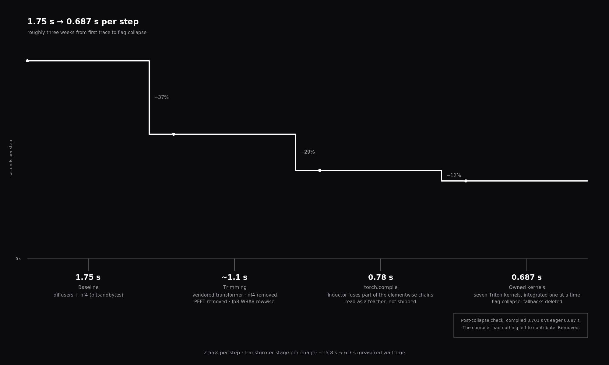1.75 s → 0.687 s per step, roughly three weeks from first trace to flag collapse. fp8 trimming took the largest single cut; torch.compile fused part of the elementwise chains; the seven owned kernels finished the job. Post-collapse, the compiled path (0.701 s) is slower than eager (0.687 s) — the compiler had nothing left to contribute.

In absolute terms: 1.75 seconds to 0.687 seconds per step, a 2.55x speedup. At 9 steps per image, the transformer stage fell from roughly 15.8 seconds to 6.7 seconds of measured wall time. On the AWS g6.xlarge billing model, this is a proportional reduction in per-image compute cost. On a service where every generation is paid for, the margin improvement is direct.

But the less visible result is what the owned kernels enable going forward. The inference path is no longer a consumer of library code. It is owned infrastructure. The same fp8 arithmetic that runs inference is the arithmetic the training backward passes run on. The LoRA hot-swap is a buffer copy into preallocated tensors, not a library call. Adding a new conditioning signal, changing the noise schedule, or running a different attention variant is a code change in the kernel files, not a negotiation with a framework’s extension API.

The backward kernels already exist, seven of them, and they have carried one complete LoRA training run end-to-end on the same fp8 arithmetic. A correctness milestone, not an operational one: the training path still has distance to cover before it meets its own criteria. But this was never only about inference speed. It was about owning the surface where the model meets the hardware, so that every direction, forward and backward, inference and training, runs on the same code, the same arithmetic, at the same precision.